Catastrophic forgetting in Lifelong learning

Learning throughout life is a sign of intelligence. Humans are always learning and adapting to life. We keep acquiring knowledge and experiences as we go along.

A machine learning model should be able to do the same. They should be able to learn new tasks as it comes along. In principle, a model should use the knowledge acquired from the previous tasks to learn a new task more effectively. It should not completely forget the old tasks as well.

Deep neural networks are one of the best learning models we have at the moment. But they tend to forget old tasks when learning a new one. They forget almost all of it - so much so we have a name for this phenomenon.

Table of Contents

Catastrophic forgetting?

Let’s define a sequence of tasks as

$$T_1, T_2, \dots, T_j, \dots,T_k$$

Each task $T_j$ consists of some training examples ${ (x^j_i, y^j_i) }^n_{i=1}$. To perform a task $T_j$, we must learn a function that maps the input $x^j_i \in \mathcal{X}^j$ to its target output $y^j_i \in \mathcal{Y}^j$. We define a deep neural network $f_\theta$ with parameters $\theta$ that learns this mapping $f_\theta:\mathcal{X}^j \rightarrow \mathcal{Y}^j$ by minimizing the loss function $l(f(x^j_i),y^j_i)$ between its prediction $f(x^j_i) \in \mathcal{Y}^j$ and target $y^j_i \in \mathcal{Y}^j$.

While the model trains on the stream of task examples $$(x^1_1, y^1_1),\dots,(x^j_i, y^j_i),\dots,(x^k_n, y^k_n)$$ we measure the average accuracy $a^j_i$ of the model on a validation set. The validation set consists of examples from all the tasks. As training progresses, we would like to see the validation accuracy grow. If the model keeps learning new tasks without forgetting old ones, it should perform better and better on the validation set. In the ideal case, the validation accuracy $a^j_i$ must increase monotonically as the number of examples $i$ and the number of tasks $t$ increase. In practice, we observe something else.

Training BERT on a sequence of tasks

Let’s take the lifelong text classification benchmark set by d’ Autume et al. (2019). It consists of five text classification datasets. Classification on each dataset is considered a distinct task $T_j$. We take the sequence ¹ of five tasks $T_{j=1},\dots,T_{j=5}$ as follows:

1. Sentiment analysis on Yelp reviews with 5 classes
2. News classification on AGNews corpus with 4 classes
3. Article classification on DBpedia corpus with 14 classes
4. Sentiment analysis on Amazon reviews with 5 classes
5. QA categorization on Yahoo answers with 10 classes

For all the experiments, we take the pre-trained BERT model (bert-base-uncased) provided by the Huggingface Transformers library. We add a linear classification layer (33 classes for all 5 tasks) on top of the pre-trained model. We use the AdamW optimizer provided by the library for training with a learning rate of $3\times10^{-5}$ and a batch size of 30.

We record the average accuracy on the validation set of all tasks while we train the model sequentially. As mentioned earlier, we expect the validation accuracy to grow. However, the experiment doesn’t match our expectations.

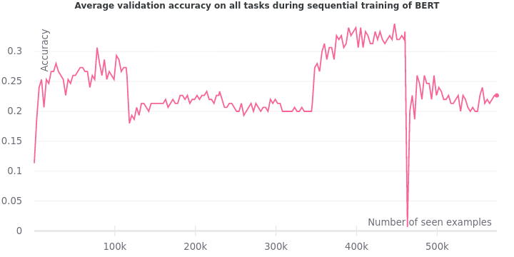
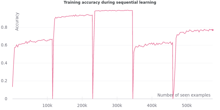
The validation accuracy not only fails to grow steadily, but it also drops sharply whenever a new task is encountered. The training accuracy plummets exactly when the model sees an example from a new task. All these precipitous drops are signs of catastrophic forgetting.

How to learn without forgetting?

In this post, we will look at some of the popularly proposed solutions to catastrophic forgetting. In particular, the focus will be on meta-learning methods. We will study their efficacy by doing our experiments and interpreting the results in the context of the relevant literature. We shall also experiment with the latest ideas on using Adapters for this problem.

Bounding the Lifelong learning problem

First, we need to establish some baselines to serve as points of comparison. As shown in the earlier experiment , sequentially training a model sets the lower bound of performance on this lifelong learning problem. Now we must identify the upper bound of performance.

In the ideal case, all the tasks would be known to us from the beginning. All the training data from these tasks would be available at once. A model can learn to optimize its performance on all tasks on average.
The scenario described above is analogous to multi-task learning. In multi-task learning, a model learns to perform multiple tasks at once. Hence, we set the multi-task performance as the upper bound on the lifelong learning problem.

We train BERT with the same setup as above except using multi-task learning. We record the average validation accuracy on all tasks when BERT is being trained on all of them together. The figure below presents the upper bound of multi-task learning against the lower bound of sequential learning.

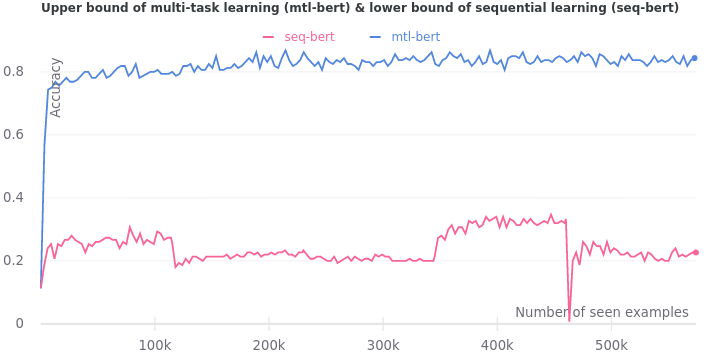
As expected, we observe no signs of catastrophic forgetting during multi-task learning. There are no precipitous drops since all tasks are made available at once. The validation accuracy rises way beyond that of sequential learning and plateaus at around 0.85.

Experience replay: bring back the i.i.d. assumption!

One of the reasons for catastrophic forgetting could be the breakdown of the i.i.d. assumption. The generic supervised learning framework assumes that each example $(x^j_i, y^j_i)$ is an identically and independently distributed (i.i.d.) sample from the probability distribution of task $T_j$. In lifelong learning, however, the stream of task examples are not i.i.d. since they are correlated. We observe a whole sequence of examples from the current task before a new task is streamed. The examples $(x^j_i, y^j_i)$ are locally correlated by the task $T_j$. How do we bring back the i.i.d. property? Experience replay.

Experience replay is about storing some of the examples seen during training. These past “experiences” are then randomly replayed by training the model on them from time to time. The frequency of re-training on some random sample from past examples decides the sparsity of experience replay. At the maximal replay frequency - training on random examples from the previous tasks at every other step - we approximate the i.i.d. assumption.

We train BERT on the sequential learning setup but with experience replay. Each training step consists of 30 examples (batch size) from the current task. The replay frequency is set to 320 steps. The number of replay examples to sample from memory is set to 96. Thus, after training on 9,600 examples from the current task we re-train the model on a sample of 96 examples from the past tasks.

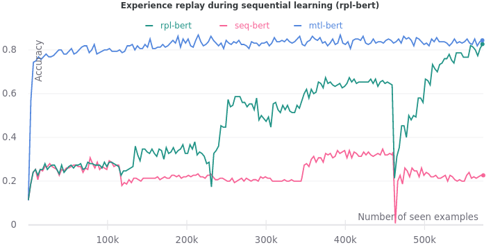
As new tasks are introduced, we see that the average validation accuracy increases in aggregate. In the end, validation accuracy (0.82) comes close to the upper bound (0.84). However, the precipitous drops remain at steps where a new task is introduced. The problem of catastrophic forgetting is not completely solved yet.

Learning to adapt

The standard procedure to fine-tune pre-trained models for new tasks is to stack a classifier at the end of the model. That’s what we did with the pre-trained BERT in our experiments above. For a classification task with $n$ classes, we appended a linear layer with input dimension $768$ and output dimension $n$. The linear layer works as a classifier by taking in $768$-dimensional feature vectors from BERT and transforming them into $n$-dimensional class distribution vectors.

Now, we know from experience that deep learning models tend to learn general features at the beginning of the network. These are then transformed into task-specific features towards the end. One of the reasons for catastrophic forgetting might be the lack of generalization. Perhaps the features learnt by the early layers of pre-trained BERT are not general enough. Can we fine-tune a pre-trained model better by injecting trainable layers within the model instead of stacking them at the end?

Adapters

Enter adapters by Houlsby et al. (2019). Adapters are task-specific modules that are injected inside a pre-trained model. The pre-trained parameters remain frozen while the adapter parameters are trained on the new downstream task. Compared to standard fine-tuning where the pre-trained parameters are also updated, the adapter fine-tuning approach improves the time and space efficiency. For $N$ tasks, we end up with $N$ adapters which are significantly smaller in total size than $N$ fine-tuned full models.

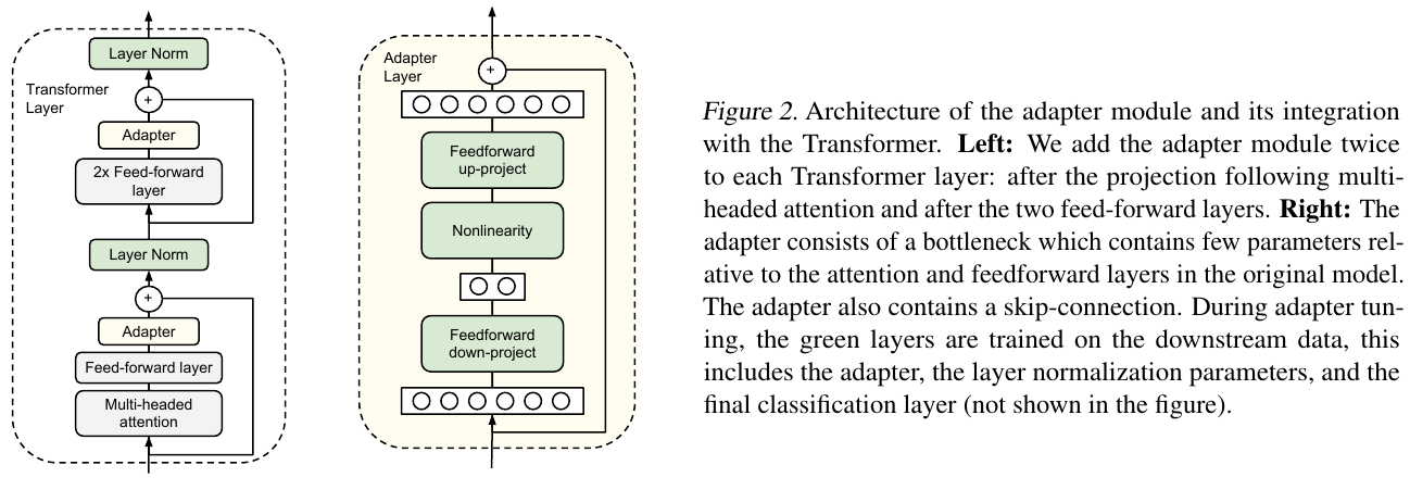
Using adapter fine-tuning of BERT, Houlsby et al. (2019). achieve similar performance to full fine-tuning ($0.4%$ difference) on the GLUE benchmark. Adapter tuning used only 1.3x parameters compared to 9x parameters when full BERT was fine-tuned on all 9 GLUE tasks. The adapters have a simple bottleneck architecture to keep the number of parameters small. They are inserted after the self-attention layer and the feed-forward layer of every transformer block. For stable training, the adapter weight initialization must be near-zero with a skip connection to approximate an identity function. It ensures that the behaviour of the modified network resembles that of the pre-trained network at the start of the training.

Now, let’s experiment with adapters to understand them better. We will contrast fine-tuning the full BERT against fine-tuning just the adapters inserted into BERT. As a control, we will fine-tune the full BERT and the adapters inserted into it. These three fine-tuning procedures will be used on our five tasks separately.

Our adapters follow the simple bottleneck architecture described in the paper. First, it projects down the hidden vectors in each BERT encoder block from $768$ dimensions to $48$ dimensions i.e. with a compression factor of $16$. Then, it is projected back up to the original $768$ dimensions.

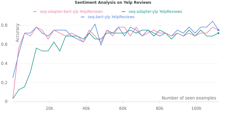
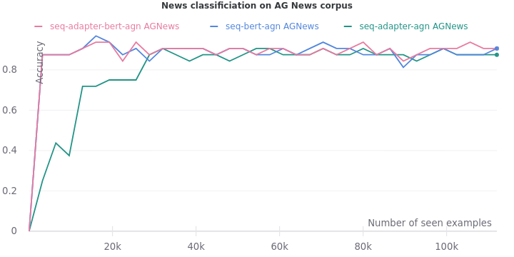
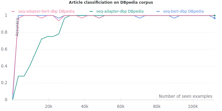
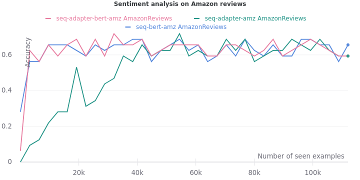
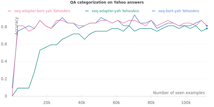
On all the five tasks, we see one consistent trend. The validation accuracy lags when only adapters are trained. But it eventually catches up when they are trained on more data.

Multi-task learning with adapters

Let’s compare the three fine-tuning procedures on all the tasks at once i.e. multi-task learning.

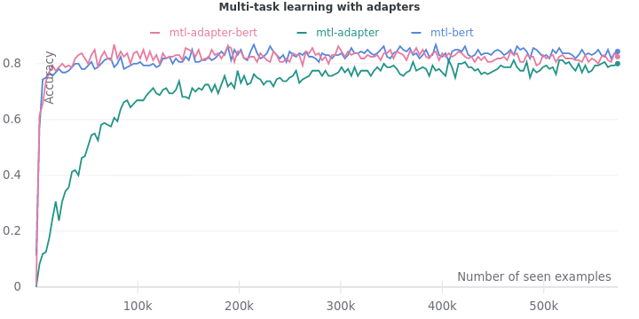
Here, we notice the same trend. Fine-tuning just the adapters requires more data to match the performance of fine-tuning the full model. Even then, the accuracy of adapter models remains slightly lower at 0.80. Fine-tuning the model and adapters achieve a final accuracy of 0.82, whereas fine-tuning the model alone reaches the final accuracy of 0.84. Surprisingly, injecting adapters into the model reduces the performance of the full model. It must be investigated further in the future.

Sequential learning with adpaters

Now, the question is can they help solve the lifelong learning problem? To see the extent of catastrophic forgetting on adapters, we run the three fine-tuning procedures on the tasks sequentially.

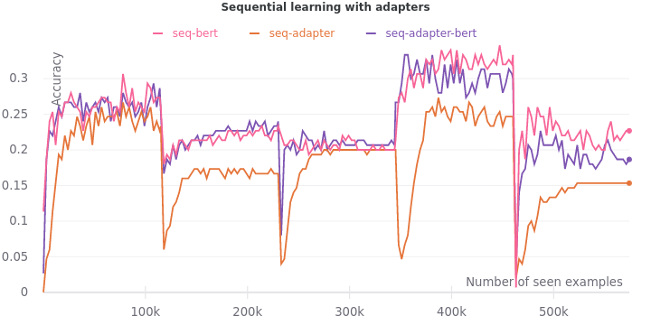
The problem has been aggravated. The accuracy during fine-tuning of adapters not only lags, but it also never catches up to the accuracy of fine-tuning full models. The final accuracy affirms the ranking of fine-tuning the full model alone (0.22) over fine-tuning both the model and adapters (0.18) over fine-tuning the adapter only (0.15).

Learning to learn

It looks like our models need a better way to adapt to new tasks. Can our models learn how to learn?

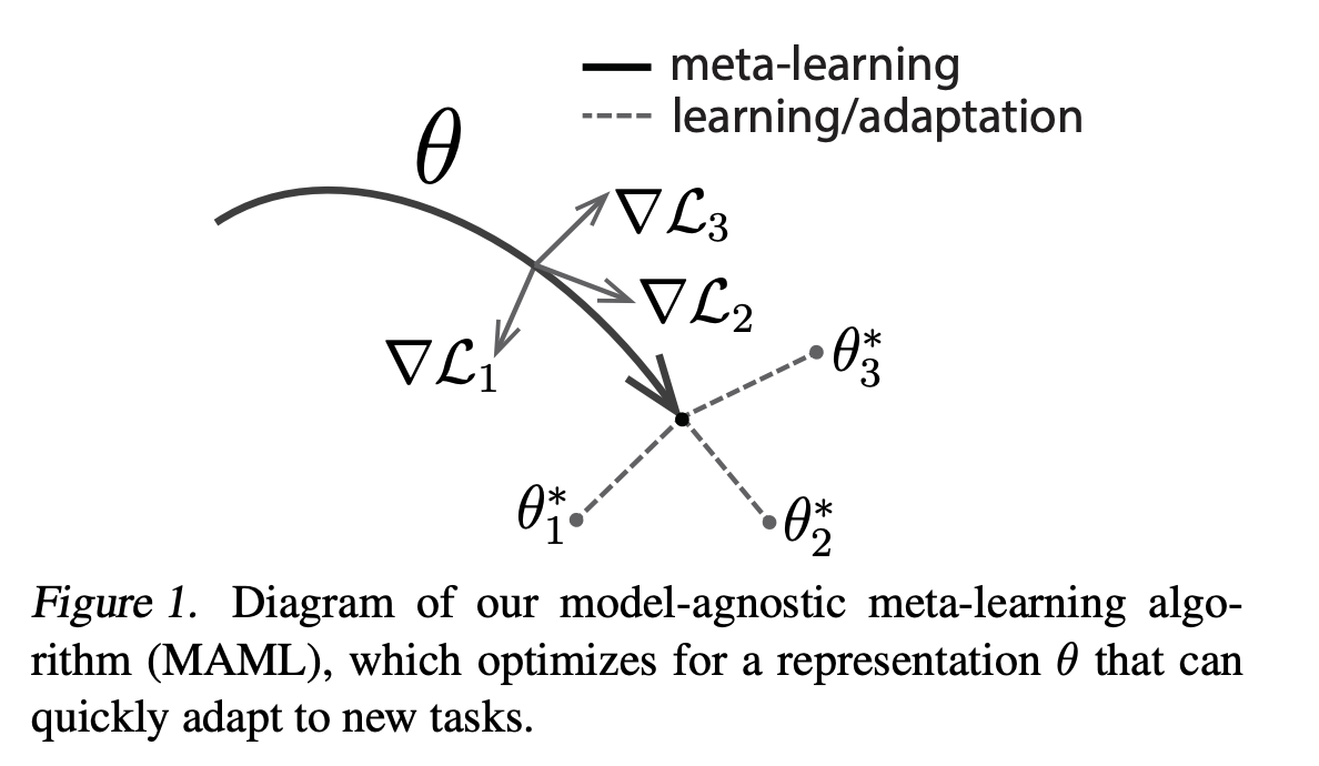
Meta-learning is about designing training procedures and models that can learn new tasks quickly. It can be used to make our models amenable to future fine-tuning. Model-agnostic meta-learning (MAML) proposed by Finn et al. (2017) is one of the most popular meta-learning methods. The article Meta-Learning: Learning to Learn Fast gives a great overview of all the popular meta-learning approaches. However, to understand MAML in-depth I encourage you to read the original paper.

In brief, MAML provides a good initialization of model parameters.
The model is led to a region in the parameter-loss landscape such that it can quickly jump to new parameters which are optimal for new tasks. The diagram of MAML shows how the model parameters $\mathbf{\theta}$ are steered towards regions which are close to the optimal parameters ${ \mathbf{\theta_1}, \mathbf{\theta_2}, \mathbf{\theta_3} }$ of three tasks.

We set the size of the support and query set to 5. Unlike the original MAML setup where the support and query set is filled up with different task examples, we fill up the support and query set from the continuous stream of task examples as they become available. The inner learning rate is set to $1\times10^{-3}$ and the outer learning rate is set to $3\times10^{-5}$. We use experience replay as described earlier.

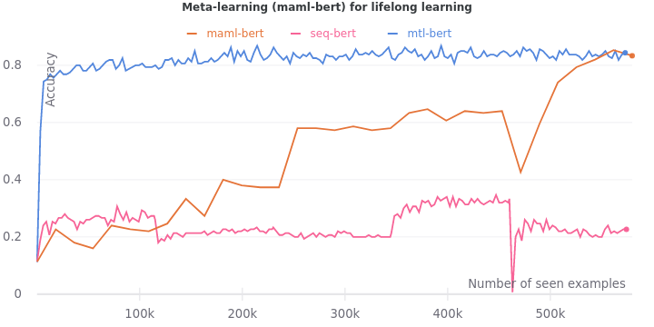
We see that the validation accuracy grows overtime to 0.83 to approach the multi-task learning accuracy at 0.84. The drops are not as extreme as it was with only experience replay. However, they still exist. Our work here is not done.

Learning to fine-tune

Can we integrate meta-learning with the idea of fine-tuning with adapters? Perhaps we could use MAML to train the adapter parameters to be more “adaptable”.

MAML on adapters

We set up the experiment with the three fine-tuning procedures described in the adapter section. But we use MAML to fine-tune them instead.

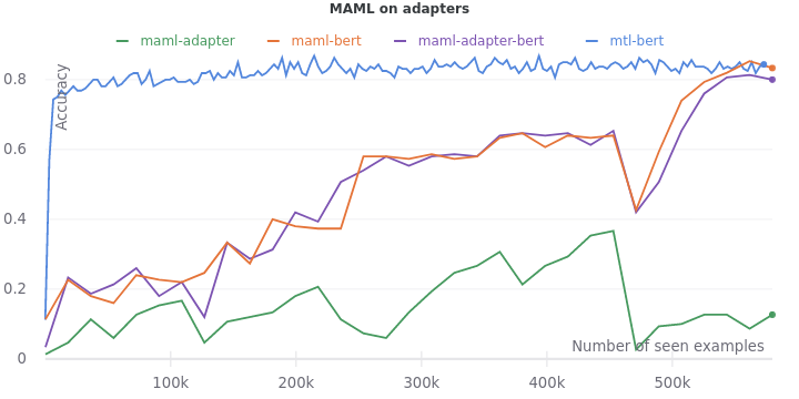
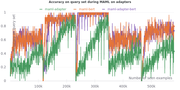
We see that the difference between fine-tuning the adapters and fine-tuning the full model is amplified when MAML is used. The final validation accuracy of fine-tuning the adapters only is an abysmal 0.12. Seems like adapters harm more than help as the fine-tuning of model and adapters leads to an accuracy (0.80) lower than that of fine-tuning just the model (0.83). Accuracy on the query sets during training tell the same story of adapters lagging, requiring more training data to catch up.

Online Meta-Learning

Perhaps, we need an objective that explicitly mitigates interference in the feature representations. The Online Meta-Learning algorithm proposed by Javed & White (2019) try to learn representations that are not only adaptable to new tasks (meta-learning) but also robust to forgetting under online updates of lifelong learning.

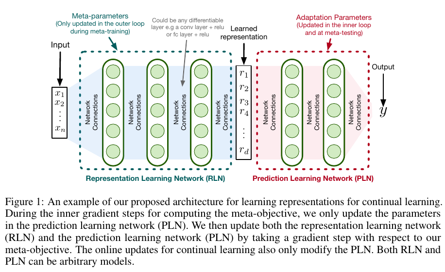
In OML, we have a Representation Learning Network (RLN) and a Prediction Learning Network (PLN). The RLN is trained in the outer loop of meta-training to learn meta-representations that are generalizable across tasks. The PLN is trained in the inner loop of meta-training (and at meta-test time) to learn the current task predictions given meta-representations from RLN. The key difference between MAML and OML is that MAML perform $l$ inner updates on the same batch but OML performs one inner update for each of the $l$ batches sampled from the task stream. For more details, please read the original paper.

Now let’s experiment with this idea. We will use OML to fine-tune a pre-trained BERT and adapters with a compression factor of 16. As a control, we will fine-tune a pre-trained BERT and adapters with a compression factor of 768 i.e. full compression such that the adapters are unusable. The other configurations and hyper-parameters of the experiment remain the same as in the MAML experiment.

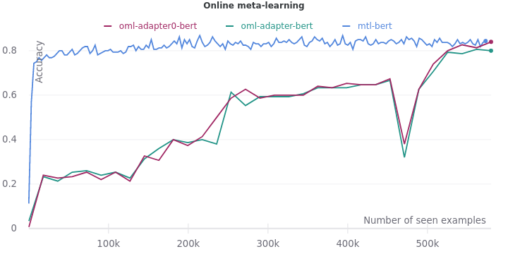
We find that even OML cannot help adapters learn better features. In fact, OML performs better on the control experiment. Fine-tuning a pre-trained BERT using OML leads to a validation accuracy of 0.84. It has finally matched the upper bound accuracy of multi-task learning.

Ablation study

Now let’s study the individual impact of the methods on catastrophic forgetting. Based on the results above, we will focus on two of the best approaches: OML and experience replay.

Impact of online meta-learning

Here, we juxtapose all the variants of meta-learning. Specifically, we want to compare the impact of meta-learning (with and without adapters) against online meta-learning (with and without adapters).

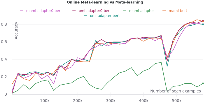
As we can see, online meta-learning doesn’t have a major impact. OML on pre-trained BERT (0.84) is only slightly better than MAML on pre-trained BERT (0.83). We should perform significance testing in the future to validate this conclusion.

Impact of meta-learning on experience replay

Now we look at the role of experience replay in mitigating catastrophic forgetting. We compare the accuracy curves when using experience replay and when using MAML with experience replay. Ideally, we should have performed another experiment using MAML without experience replay if it wasn’t for resource constraints.

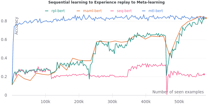
MAML seems to smoothen the accuracy curve.
The final and sharpest drop on the last task is also blunted by MAML. Overall, we find that MAML with experience replay seems to perform better than just experience replay.

To sum up, experience replay and meta-learning are effective solutions to catastrophic forgetting in lifelong learning.